Julia でニューラルネットワークを可視化してみた

はじめに

ニューラルネットの挙動を理解する：全結合層と活性化関数による変換での可視化が魅力的だったので、Julia の Flux.jl で同様のことをやってみました

ニューラルネットの挙動を理解する：全結合層と活性化関数による変換 - Qiita

前回の記事でChirstopher Colah氏の記事「ニューラルネット、多様体、トポロジー」の中のいくつかの動画を再現しました。https://qiita.com/Soichir0/items/…

https://qiita.com

問題設定

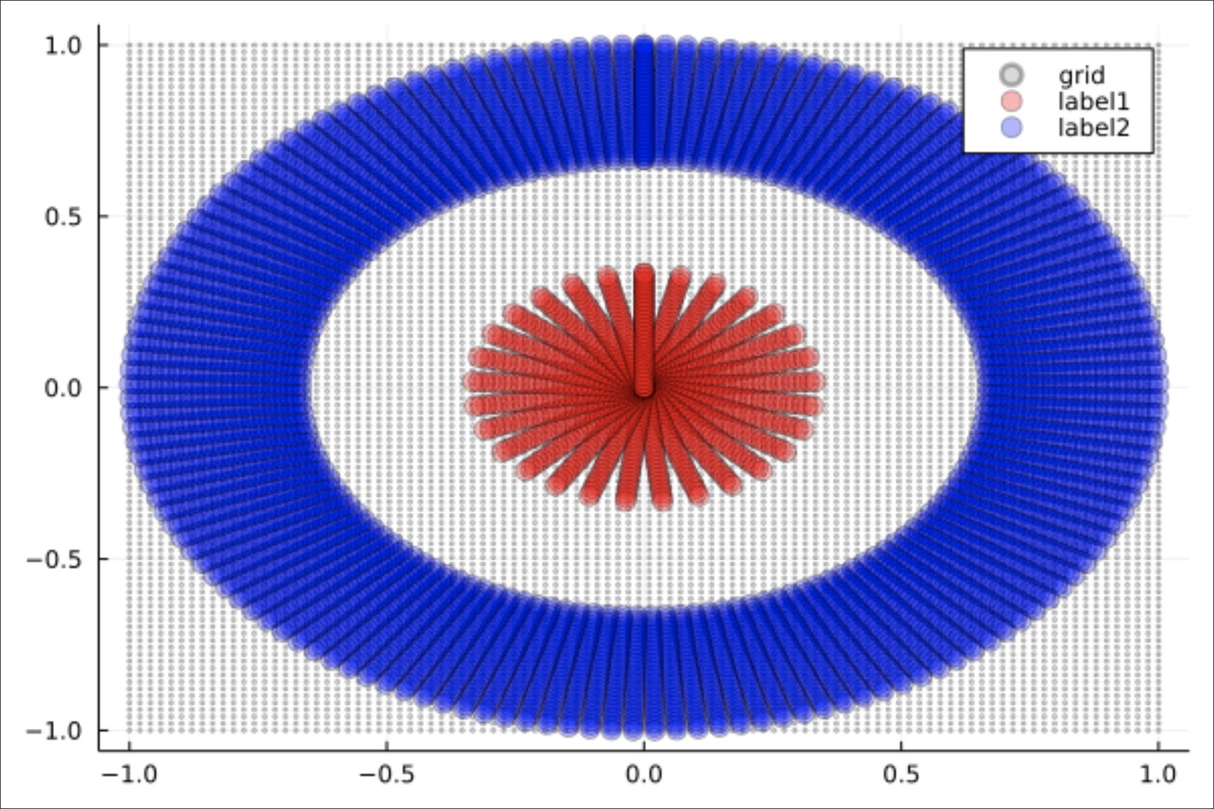
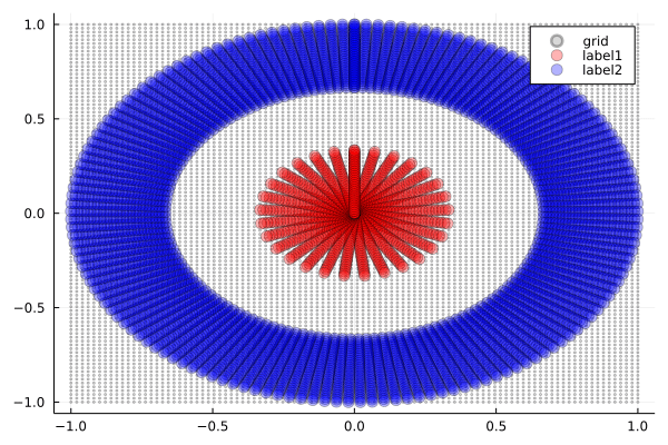
3層のニューラルネットワークで下図のデータを2値分類
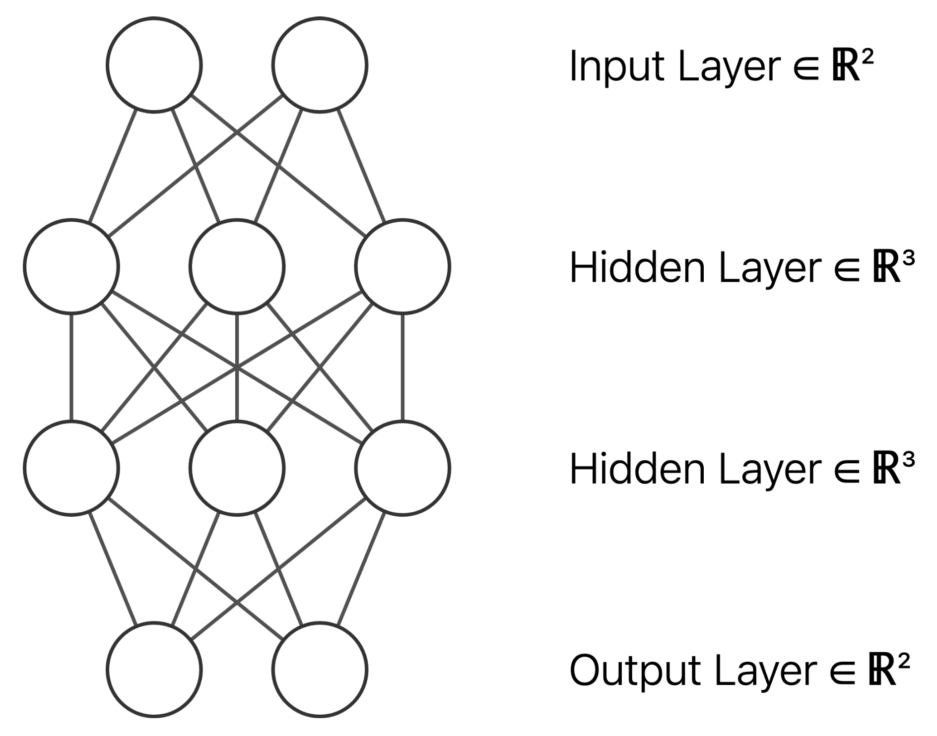
ネットワークの構造
TODO: アフィン変換をする隠れ層が入力層の直後に追加で入るにも関わらず、図に描き忘れているので修正

Julia での実装

パッケージのインポート

using Flux
using LinearAlgebra
using Plots
using ProgressMeter

訓練用の入力

# 円状に点を作成
circle_coords(r_min, r_max, r_size, θ_size) = [
    r .* (sin(θ), cos(θ))
    for θ in range(0, 2π, length=θ_size)
    for r in range(r_min, r_max, length=r_size)
]

N = 30
x_coords = [
    circle_coords(1e-3, 1 / 3, N, N),
    circle_coords(2 / 3, 1, N, N)
]
coords2mat(xs) = hcat([[xs[n]...,] for n in axes(xs, 1)]...)
x_train = (coords2mat ∘ vcat)(x_coords...);

入力に対応する教師ラベルを生成して 🚫

Post not found と結合

y_train = (coords2mat ∘ vcat)(
    [(1, 0) for _ in 1:N^2],
    [(0, 1) for _ in 1:N^2]
);
data = [(x_train, y_train)];

ニューラルネットワークを学習

# 訓練対象のモデル作成
model = Chain(
    Dense(2 => 3),
    Dense(3 => 3, relu),
    Dense(3 => 3, relu),
    Dense(3 => 2),
    softmax
)

# モデルの学習
epoch_num = 50_000;
params = Flux.params(model);
regular_rate = 0.01;
loss(x, y) = Flux.crossentropy(model(x), y) + regular_rate * norm(params);
opt = Descent()
@showprogress "Epoch of training: " for epoch in 1:epoch_num
    Flux.train!(loss, params, data, opt)
end

格子点

function grid_coords(x_coords)
    x_mat = coords2mat(x_coords)
    x₁_min, x₁_max = round.([minimum(x_mat[1, :]), maximum(x_mat[1, :])])
    x₂_min, x₂_max = round.([minimum(x_mat[2, :]), maximum(x_mat[2, :])])
    [
        Float64.((i, j))
        for i in range(x₁_min, x₁_max, length=100)
        for j in range(x₂_min, x₂_max, length=100)
    ]
end

🚫

Post not found , 🚫

Post not found を線形補間する関数の定義
また，中間層の出力は最初の2次元のみ表示に用いる

# リストの隣接する要素の平均値をその要素間に挿入
insert_lerp(xs) =
    let xs_lerp = [
            [
                (xs[n][i] .+ xs[n+1][i]) ./ 2
                for i in axes(xs[n], 1)
            ]
            for n in axes(xs, 1)[1:end-1]
        ]
        [
            n % 2 == 0 ? xs_lerp[div(n, 2)] : xs[div(n, 2)+1]
            for n in 1:2size(xs, 1)-1
        ]
    end

# GIF生成のためのフレームを作成
# フレーム数はおよそ 2^log2_expansion_rate 倍となる
function create_frames(x_coords, log2_expansion_rate=6)
    x_mat = coords2mat(x_coords)
    anim_x = [x_coords]
    for layer_depth in 1:length(model)
				mat2coords(xs) = [(xs[:, j]...,) for j in axes(xs, 2)]
        y = model[1:layer_depth](x_mat)[1:2, :] # 最初の2次元をプロットに使用
        y_coords = mat2coords(y)
        anim_x = [anim_x..., y_coords]
    end
    foldl(∘, repeat([insert_lerp], log2_expansion_rate))(anim_x)
end

Plots の @gif マクロでアニメーションを生成

# 訓練結果のブロット
x_plot = [
    circle_coords(1e-3, 1 / 3, N, N),
    circle_coords(2 / 3, 1, N, 5N)
];
anim_xplot = create_frames.(x_plot);

# 格子点のプロット
anim_xgrid = (create_frames ∘ grid_coords ∘ vcat)(x_plot...);

# プロット用の点をまとめる
anim_plots = zip(anim_xplot..., anim_xgrid);

gif_prog = Progress(length(anim_plots), desc="Render GIF: ");
@gif for (x₁, x₂, xgrid) in anim_plots
    plot()
    plot!(xgrid, seriestype=:scatter, mc=:gray, ma=0.3, ms=2, label="grid")
    plot!(x₁, seriestype=:scatter, mc=:red, ma=0.3, ms=6, label="label1")
    plot!(x₂, seriestype=:scatter, mc=:blue, ma=0.3, ms=6, label="label2")
    next!(gif_prog)
end

ソースコード全体

using Flux
using LinearAlgebra
using Plots
using ProgressMeter

coords2mat(xs) = hcat([[xs[n]...,] for n in axes(xs, 1)]...)
mat2coords(xs) = [(xs[:, j]...,) for j in axes(xs, 2)]

insert_lerp(xs) =
    let xs_lerp = [
            [
                (xs[n][i] .+ xs[n+1][i]) ./ 2
                for i in axes(xs[n], 1)
            ]
            for n in axes(xs, 1)[1:end-1]
        ]
        [
            n % 2 == 0 ? xs_lerp[div(n, 2)] : xs[div(n, 2)+1]
            for n in 1:2size(xs, 1)-1
        ]
    end

function create_frames(x_coords, log2_expansion_rate=6)
    x_mat = coords2mat(x_coords)
    anim_x = [x_coords]
    for layer_depth in 1:length(model)
        y = model[1:layer_depth](x_mat)[1:2, :]
        y_coords = mat2coords(y)
        anim_x = [anim_x..., y_coords]
    end
    foldl(∘, repeat([insert_lerp], log2_expansion_rate))(anim_x)
end

# 格子点を作成
function grid_coords(x_coords)
    x_mat = coords2mat(x_coords)
    x₁_min, x₁_max = round.([minimum(x_mat[1, :]), maximum(x_mat[1, :])])
    x₂_min, x₂_max = round.([minimum(x_mat[2, :]), maximum(x_mat[2, :])])
    [
        Float64.((i, j))
        for i in range(x₁_min, x₁_max, length=100)
        for j in range(x₂_min, x₂_max, length=100)
    ]
end

# 円状に点を作成
circle_coords(r_min, r_max, r_size, θ_size) = [
    r .* (sin(θ), cos(θ))
    for θ in range(0, 2π, length=θ_size)
    for r in range(r_min, r_max, length=r_size)
]

# 訓練データの作詞
N = 30
x_coords = [
    circle_coords(1e-3, 1 / 3, N, N),
    circle_coords(2 / 3, 1, N, N)
]
x_train = (coords2mat ∘ vcat)(x_coords...);
y_train = (coords2mat ∘ vcat)(
    [(1, 0) for _ in 1:N^2],
    [(0, 1) for _ in 1:N^2]
);
data = [(x_train, y_train)];

# 訓練対象のモデル作成
model = Chain(
    Dense(2 => 3),
    Dense(3 => 3, relu),
    Dense(3 => 3, relu),
    Dense(3 => 2),
    softmax
)

# モデルの学習
epoch_num = 50_000;
params = Flux.params(model);
regular_rate = 0.01;
loss(x, y) = Flux.crossentropy(model(x), y) + regular_rate * norm(params);
opt = Descent()

@showprogress "Epoch of training: " for epoch in 1:epoch_num
    Flux.train!(loss, params, data, opt)
end

# 訓練結果のブロット
x_plot = [
    circle_coords(1e-3, 1 / 3, N, N),
    circle_coords(2 / 3, 1, N, 5N)
];
anim_xplot = create_frames.(x_plot);
anim_xgrid = (create_frames ∘ grid_coords ∘ vcat)(x_plot...);
anim_plots = zip(anim_xplot..., anim_xgrid);
gif_prog = Progress(length(anim_plots), desc="Render GIF: ");
@gif for (x₁, x₂, xgrid) in anim_plots
    plot()
    plot!(xgrid, seriestype=:scatter, mc=:gray, ma=0.3, ms=2, label="grid")
    plot!(x₁, seriestype=:scatter, mc=:red, ma=0.3, ms=6, label="label1")
    plot!(x₂, seriestype=:scatter, mc=:blue, ma=0.3, ms=6, label="label2")
    next!(gif_prog)
end